.svg)
At Sift, we believe that engineers can only be as effective as the data which is discoverable to them. For teams building complex hardware (spaceships, planes, drones, vehicles, etc.), it’s all too common for telemetry data to be locked behind rigid schema definitions or buried in SQL-based dashboards. In order for hardware engineering teams to guarantee safety and performance, engineers need data infrastructure and a UX that makes their telemetry data discoverable, intuitive, and fast. Furthermore, for data infrastructure to be suitable for mission-critical hardware, it needs to be rugged enough to handle data from millions of sensors. This post outlines how Sift approaches UX and how we built a data architecture that lets you get the most out of your telemetry sensor data.
Your team's velocity depends on its ability to make information discoverable
“Making your data accessible to every engineer” is something that reads great on the slide deck and sounds easy in concept, but is a surprisingly difficult UX challenge. Most open-source telemetry tools were built by and for software engineers. (Frequently not the hardware engineers that actually have to use them!) Dashboards often assume the user knows what channels for sensor data exist, what they’re called, and how to write the right SQL or Flux syntax to query them. This is especially true of tools like Grafana or Influx. But in real-world environments, users often aren’t the authors of the data. For example, what if a GNC engineer is inspecting a failed propulsion test? Or a power test technician on the factory floor finds unexplained thermal anomalies? You’re stuck if you don’t already know the exact name of a channel, or worse, if the schema changed with the latest software release. Collaborative velocity across teams becomes beholden to support tickets. This is unacceptable in modern hardware orgs where cross-functional debugging is the norm, not the exception.

To keep the context the engineer needs at their fingertips, Sift went from BORG to better
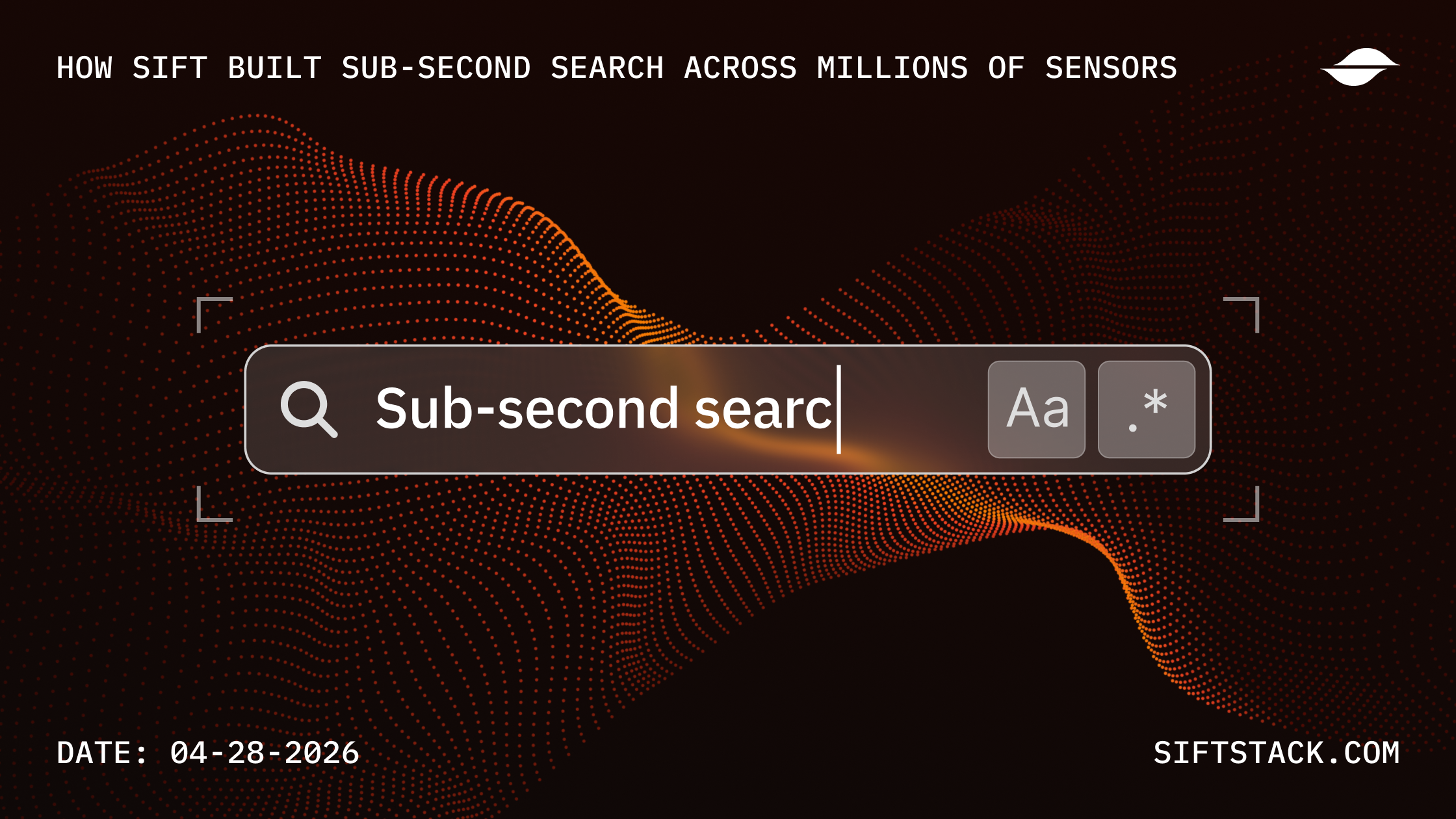
Engineers deserve better than searching for schema they didn’t write or waiting eons for a dropdown to load thousands if not millions of channels. So when we built Sift, we knew that we wanted to offer the best-in-class UX, inspired by the tooling we worked with at SpaceX (BORG). To do this, we built discoverability into Sift’s DNA by supporting pattern matching and making metadata searchable, all without compromising performance.
Pattern matching
Key to any discoverable performance search is supporting pattern matching. In many cases, users might remember portions of channel names, but not the exact name or spelling. Pattern matching enables users to type RO ER to successfully return ROVER. Additionally, this would also be helpful in instances where users are looking for multiple sensors of the same category but don’t want to have to type the full name of each sensor. For example, a GNC engineer trying to debug inertial measurement units (IMUs) would probably prefer to type “gnc imu” instead of having to remember naming conventions and syntax to find “gnc.flight_computer1.imu3” and its related IMUs. Pattern matching supports discoverability by aligning with how engineers remember information practically and adds the convenience of not having to type all of the interim information for every search.

Searchable metadata
But discoverability needs to go beyond convenience or returning results on partial keyword matches. What happens if engineers are trying to explore subsystems with which they’re completely unfamiliar? For example, what if a thermal engineer is trying to review mechanical test logs. To support this, Sift made metadata searchable. In a scenario where the thermal engineer is trying to validate that components remained within thermal limits during a vibration test, they could query for metadata tags like “vibe test,” or “thermal,” to find “payload_mountbracket2” that collects data from vibration tests or logs data in °C. This kind of metadata-driven search unlocks cross-team collaboration, speeds up incident response, and reduces reliance on tribal knowledge.
Building telemetry data architecture from scratch
To query their telemetry data, most teams start with a familiar pattern: add a search bar to the UI, maybe offer a few filters, and wire that up to a simple query on the backend. The implementation usually indexes basic metadata (such as names, descriptions, tags) and supports pattern matching queries using multiple sub-string matches or regular expressions. However, without appropriate indexing strategies, this implementation results in degraded performance. This degradation is further compounded as hardware iterates and the number of subsystems grows. As hardware becomes more complex, the number of sensors and associated telemetry data grows exponentially. Search performance, already struggling with a more complex machine, can only get worse as teams build multiple assets or God forbid need to manage an entire fleet of different kinds of assets. As sensors and thus telemetry data needs scale, queries degrade. Tail latencies spike. And most critically, the global indexes in a simple architecture can’t keep up.
Hardware engineers need to be able to quickly find their data while searching through millions of sensors. And anyone working on the test bench needs to be able to make decisions in real-time. How can you provide the robust architecture and snappy search performance that these workflows so desperately need?
If you were to build out an architecture to get a quick telemetry prototype off the ground, you might use PostgreSQL to bootstrap something simple like this:
CREATE USER my_user;
CREATE DATABASE Sift WITH owner = 'my_user';

CREATE TABLE organizations (
  organization_id UUID PRIMARY KEY DEFAULT gen_random_uuid(),
  name TEXT NOT NULL
);


CREATE TABLE assets (
  asset_id UUID PRIMARY KEY DEFAULT gen_random_uuid(),
  name TEXT NOT NULL,
  organization_id UUID NOT NULL,
  FOREIGN KEY (organization_id) REFERENCES organizations(organization_id)
);

CREATE TABLE channels (
  channel_id UUID PRIMARY KEY DEFAULT gen_random_uuid(),
  name TEXT,
  organization_id UUID NOT NULL,
  FOREIGN KEY (organization_id) REFERENCES organizations(organization_id),
  asset_id UUID NOT NULL,
  FOREIGN KEY (asset_id) REFERENCES assets(asset_id)
);

-- Where assets refer to any hardware machine (rover, satellite, drone, car, etc.) that produces time-series telemetry data and channels refer to the asset's sensors that measure telemetry data. Examples of sensor data collected in channels include temperature, pressure, humidity, battery levels, stateful data, etc. More assets and/or sensors = more channels.
In this particular example, we seeded the database with a few assets with wildly different channel counts for its sensor data. Here, the asset MarsRover1 has just 1,000 channels but asset MarsRover 4 has a million:
SELECT
    assets.asset_id,
    assets.name,
    COUNT(*) AS channels_count
FROM assets
INNER JOIN channels ON assets.asset_id = channels.asset_id
GROUP BY assets.asset_id
"asset_id"    "name"    "channels_count"
"2ecc5583-5007-4177-a81e-12da5c65424f"    "MarsRover3"    45000
"990790fa-aad9-4106-9dd2-2ccf6c1f3dcd"    "MarsRover2"    45000
"affda90b-f16e-47c8-a4de-fb6099a8abdf"    "MarsRover1"    1000
"b69535fe-2a46-4d6c-88fc-402b2d7dee95"    "MarsRover4"    1000000
If you were to query with a baseline Regex search, you’d find that the scan is costly and slow, especially on your more complex machine with the most sensors:
-- Query on asset with 1,000,000 channels
EXPLAIN ANALYZE
SELECT *
FROM channels
WHERE
    asset_id = 'b69535fe-2a46-4d6c-88fc-402b2d7dee95'
    AND name ~ 'channel_11\d{2}2$'
QUERY PLAN
Seq Scan on channels  (cost=10000000000.00..10000030882.00 rows=100 width=73) (actual time=111.087..1008.285 rows=100 loops=1)
  Filter: ((name ~ 'channel_11\d{2}2$'::text) AND (asset_id =
'b69535fe-2a46-4d6c-88fc-402b2d7dee95'::uuid))
  Rows Removed by Filter: 1090900
Planning Time: 0.501 ms
Execution Time: 1008.299 ms
In an attempt to improve search performance, a common approach is to add the pg_trgm extension and create a GIN index (or GiST depending on how often your data changes):
CREATE EXTENSION pg_trgm;
CREATE INDEX channels_name_trgm_idx ON channels USING GIN (name gin_trgm_ops);


-- Query on asset with 1,000,000 channels
EXPLAIN ANALYZE
SELECT *
FROM channels
WHERE
    asset_id = 'b69535fe-2a46-4d6c-88fc-402b2d7dee95'
    AND name ~ 'channel_11\d{2}2$'
QUERY PLAN
Bitmap Heap Scan on channels  (cost=164.84..574.14 rows=100 width=73) (actual time=18.801..37.540 rows=100 loops=1)
  Recheck Cond: (name ~ 'channel_11\d{2}2$'::text)
  Rows Removed by Index Recheck: 13044
  Filter: (asset_id =
'b69535fe-2a46-4d6c-88fc-402b2d7dee95'::uuid)
  Rows Removed by Filter: 200
  Heap Blocks: exact=192
  ->  Bitmap Index Scan on channels_name_trgm_idx  (cost=0.00..164.82 rows=109 width=0) (actual time=10.522..10.522 rows=13344 loops=1)
        Index Cond: (name ~ 'channel_11\d{2}2$'::text)
Planning Time: 1.201 ms
Execution Time: 37.597 ms
Using this new index, the query is much faster and the cost is significantly reduced.
Before pg_trgm GIN index:
- Plan: Full sequential scan on 1M rows
- Execution Time: 1008ms
After pg_trgm GIN index:
- Plan: Bitmap index scan via trigram
- Execution Time: 37ms (more than 27x faster!)
It looks like the pg_trgm GIN index improved search performance. But is it robust and consistent? Now that we’ve queried an asset with many channels, let’s query an asset with just a few channels:
-- Query on asset with 1,000 channels
EXPLAIN ANALYZE
SELECT *
FROM channels
WHERE
    asset_id = 'affda90b-f16e-47c8-a4de-fb6099a8abdf'
    AND name ~ 'channel_1\d{2}1'
QUERY PLAN
Bitmap Heap Scan on channels  (cost=222.65..14564.38 rows=11 width=73) (actual time=1155.408..1155.408 rows=0 loops=1)
  Recheck Cond: (name ~ 'channel_1\d{2}1'::text)
  Rows Removed by Index Recheck: 1077700
  Filter: (asset_id =
'affda90b-f16e-47c8-a4de-fb6099a8abdf'::uuid)
  Rows Removed by Filter: 13300
  Heap Blocks: exact=14517
  ->  Bitmap Index Scan on channels_name_trgm_idx  (cost=0.00..222.65 rows=11020 width=0) (actual time=131.078..131.078 rows=1091000 loops=1)
        Index Cond: (name ~ 'channel_1\d{2}1'::text)
Planning Time: 0.657 ms
Execution Time: 1155.450 ms
Notice that searching inside a small asset with only 1000 channels can be slower than a large one with 1000000 channels (1.1 second scan vs 0.4 second scan). When you are discovering telemetry for a specific channel of sensor data, it’s almost always in the context of a particular asset or hardware unit that we are interested in. Right now the global channel count for an organization affects searching for channels across every asset which is detrimental to performance.
To fix this, one might add a B-tree index on asset_id to leverage multiple indexes and scope search to a single asset:
CREATE INDEX channels_asset_id_idx ON channels (asset_id);
This helps. PostgreSQL will use the index to quickly scope the relevant asset. The resulting query plan:
-- Query on asset with 1,000 channels
EXPLAIN ANALYZE
SELECT *
FROM channels
WHERE
    asset_id = 'affda90b-f16e-47c8-a4de-fb6099a8abdf'
    AND name ~ 'channel_1\d{2}1'
QUERY PLAN
Index Scan using channels_asset_id_idx on channels  (cost=0.43..52.70 rows=11 width=73) (actual time=3.877..3.877 rows=0 loops=1)
  Index Cond: (asset_id =
'affda90b-f16e-47c8-a4de-fb6099a8abdf'::uuid)
  Filter: (name ~ 'channel_1\d{2}1'::text)
  Rows Removed by Filter: 1000
Planning Time: 1.482 ms
Execution Time: 3.894 ms
We’ve significantly reduced the cost of the query but there’s another problem: we’re no longer using our trigram GIN index. This is because PostgreSQL’s query planner has deemed that consulting just channels_asset_id_idx is faster than consulting multiple indexes, likely because of the low channel count. Let’s try an asset with a larger channel count:
-- Query on asset with 45,000 channels
EXPLAIN ANALYZE
SELECT *
FROM channels
WHERE
    asset_id = '2ecc5583-5007-4177-a81e-12da5c65424f'
    AND name ~ 'channel_4\d{3}1'
QUERY PLAN
Bitmap Heap Scan on channels  (cost=140.82..550.12 rows=4 width=73) (actual time=208.199..1158.741 rows=500 loops=1)
  Recheck Cond: (name ~ 'channel_4\d{3}1'::text)
  Rows Removed by Index Recheck: 1079000
  Filter: (asset_id =
'2ecc5583-5007-4177-a81e-12da5c65424f'::uuid)
  Rows Removed by Filter: 11500
  Heap Blocks: exact=14517
  ->  Bitmap Index Scan on channels_name_trgm_idx  (cost=0.00..140.82 rows=109 width=0) (actual time=130.231..130.232 rows=1091000 loops=1)
        Index Cond: (name ~ 'channel_4\d{3}1'::text)
Planning Time: 0.741 ms
Execution Time: 1158.814 ms
Given that we’re now doing pattern matching on an asset with a higher channel count, PostgreSQL is now preferring using the trigram index and we’re not leveraging our B-tree index. This brings us back to the original problem of searches being affected by the global channel count for all assets across the organization.
As the amount of assets increases, PostgreSQL could eventually leverage both indexes, for consistency’s sake, some people may prefer a general indexing strategy that works all the time. So how could you accomplish this?
The best of both worlds
To create a query plan that can leverage the best of both indexes consistently, you could create a hybrid index using btree_gin:
Let’s create a new index:
CREATE EXTENSION btree_gin;

CREATE INDEX channels_asset_id_btree_name_trgm_idx
    ON channels
    USING GIN (asset_id, name gin_trgm_ops);


-- Has 45,000 channels
EXPLAIN ANALYZE
SELECT *
FROM channels
WHERE
    asset_id = '2ecc5583-5007-4177-a81e-12da5c65424f'
    AND name ~ 'channel_4\d{3}1'
QUERY PLAN
Bitmap Heap Scan on channels  (cost=164.05..179.91 rows=4 width=73) (actual time=60.889..67.507 rows=500 loops=1)
  Recheck Cond: ((asset_id =
'2ecc5583-5007-4177-a81e-12da5c65424f'::uuid) AND (name ~
'channel_4\d{3}1'::text))
  Rows Removed by Index Recheck: 44500
  Heap Blocks: exact=591
  ->  Bitmap Index Scan on channels_asset_id_btree_name_trgm_idx  (cost=0.00..164.04 rows=4 width=0) (actual time=18.694..18.694 rows=45000 loops=1)
        Index Cond: ((asset_id = '2ecc5583-5007-4177-a81e-12da5c65424f'::uuid) AND (name ~
'channel_4\d{3}1'::text))
Planning Time: 0.820 ms
Execution Time: 67.547 ms
From 1158.814 ms to 67.547 ms. That’s a serious performance boost. With this strategy we’ve effectively implemented a fast pattern matching strategy in PostgreSQL that allows search through an asset’s channels. A growing number of sensors over time will not cause performance degradations across all assets.
With that we can go ahead and drop our original B-tree and GIN-trigram index:
DROP INDEX channels_name_trgm_idx;
DROP INDEX channels_asset_id_idx;Delivering 20x faster performance so the information you need is always at your fingertips
In our example query plan:
- Execution time drops from 1158ms → 67ms (almost 20x faster!)
- Query plan confirms use of both asset filtering and trigram search
In Sift’s actual deployments:
- Sift’s customer with the most channels is Parallel Systems which has ~200 million channels across its library
- Sift maintains sub-second query speeds across Parallel with ~200 million sensors
- Parallel’s highest-cardinality asset has almost 45000 sensors alone
Building for the future
Of course, designing a performant search experience is only part of the challenge. Ensuring that UX stands the test of time is equally critical. As hardware systems evolve, so too do their telemetry schemas, naming conventions, and sensor definitions. A robust telemetry platform must support both legacy and future-facing data models side by side, often within the same interface. The teams on the bleeding edge of modern machines aren’t just trying to build for the next 5 years, they need their next-generation hardware to support 20 year missions. Sift’s data architecture and UX is built to enable your machines to stand the test of time.
Want your engineers spending less time searching for context and more time building? We'd love to hear from you.